Introduction • RSVsim

library(RSVsim)
library(ggplot2)

# specifying the some age limits to use with the model
age.limits <- c(seq(0, 2, 0.2), seq(10, 60, 20))

In this vignette, we give an overview of the mathematical model of RSV transmission and how to use this package to run the model.

Model structure

The model is an adapted version of an susceptible-exposed-infectious-recovered-susceptible (SEIRS) deterministic, ordinary differential equation (ODE) model outlined in:

Hogan, A. B., Campbell, P. T., Blyth, C. C., Lim, F. J., Fathima, P., Davis, S., … & Glass, K. (2017). Potential impact of a maternal vaccine for RSV: a mathematical modelling study. Vaccine, 35(45), 6172-6179, https://doi.org/10.1016/j.vaccine.2017.09.043,
Nazareno, A. L., Newall, A. T., Muscatello, D. J., Hogan, A. B., & Wood, J. G. (2024). Modelling the epidemiological impact of maternal respiratory syncytial virus (RSV) vaccination in Australia. Vaccine, 42(26), 126418, https://doi.org/10.1016/j.vaccine.2024.126418.

In brief, the model is age-structured and primary (the first) and secondary infections (any subsequent infection) are specifically tracked. The force of infection is determined by a seasonal forcing function and the age-specific contact matrix (the mean contacts per person).

Contact matrix

The R/RSVsim_contact_matrix.R function obtains contact matrices with age groupings that are less than one year. To do so, the socialmixr (https://epiforecasts.io/socialmixr/) package is used to obtain the contact matrix for the age groupings to the nearest whole year, using the POLYMOD data (https://doi.org/10.1371/journal.pmed.0050074). This contact matrix is calculated such that the total contacts in the population are symmetric (assuming population data from World Population Prospects of the United Nations). Within age groups less than one year, these contacts are divided evenly according to the size of the age group (in years). The function takes two arguments: (1) the country to obtain the POLYMOD contact data from and (2) the lower age limits of the age groups.

contact_population_list <- RSVsim_contact_matrix(country = "United Kingdom", age.limits = age.limits)
#> Warning in RSVsim_contact_matrix(country = "United Kingdom", age.limits = age.limits): Not all age.limits are integers.
#>             The contact matrix was calculated for the age groups given by the integers
#>             and divided uniformly within the smaller age groups.
#>             A warning from socialmixr about linearly estimating the integer age groups within the 5-year age bands will also appear.
#> Warning in pop_age(survey.pop, part.age.group.present, ...): Not all age groups represented in population data (5-year age band).
#>   Linearly estimating age group sizes from the 5-year bands.

matrix_mean_plot <- contact_population_list$matrix_mean |> 
  as.data.frame() |> 
  tibble::rownames_to_column("age_y") |> 
  tidyr::pivot_longer(-age_y, names_to = "age_x", values_to = "mean_contacts")

ggplot(data = matrix_mean_plot, 
       aes(x = age_x, y = age_y, fill = mean_contacts)) + 
  geom_tile() +
  xlab("age") + ylab("age") + theme_classic()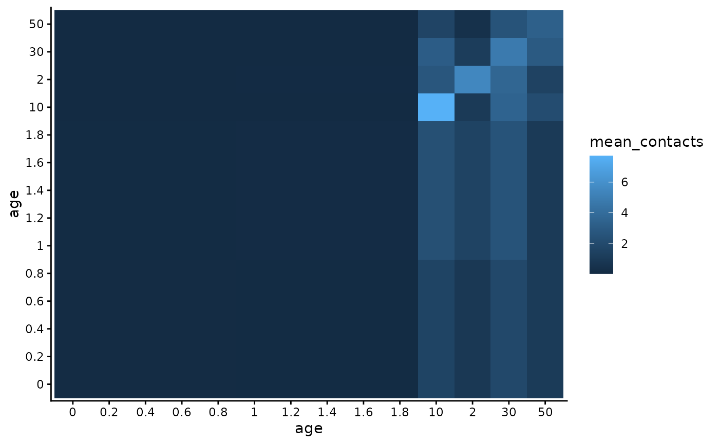

Default parameters

To obtain a list of the default parameters to run the model use the R/RSVsim_parameters.R function. The parameters can be changed by using the overrides argument; for example we override $b0$ (the transmission rate coefficient) with a value of $0.15$ .

parameters <- RSVsim_parameters(overrides = list("b0" = 0.15), 
                                contact_population_list = contact_population_list,
                                fitted = NULL)

Running the model

To run the model the R/RSVsim_run_model.R function is used. Cohort aging is used to age the population. At each time, a proportion of each cohort is aged, with this proportion determined by the length of time before people are aged (cohort_step_size) as a proportion of the total length of time in each age group. If no initial conditions are given, it is assumed there is one percent prevalence in the primary infection compartment and everyone else is susceptible to primary infection. All new borns are assumed to be susceptible to their primary infection. Below, we plot the simulated number of people that are susceptible and infected, with the line type indicating whether the infection is primary or secondary.

out <- RSVsim_run_model_dust(parameters = parameters,
                             times = seq(0, 3650, 0.25), # maximum time to run the model for
                             cohort_step_size = 10, # time at which to age people\
                             init_conds = NULL,
                             warm_up = 3650 - 365 * 3)

ggplot(data = out) +
  geom_line(aes(x = time, y = Sp), linetype = 1) +
  geom_line(aes(x = time, y = Ss), linetype = 2) +
  geom_line(aes(x = time, y = Ip), col = "skyblue", linetype = 1) +
  geom_line(aes(x = time, y = Is), col = "skyblue", linetype = 2) +
  facet_wrap(~age_chr, scales = "free_y") + theme_classic() +
  xlab("Days") +
  ylab("Number of susceptible (black) or infected (blue) people")

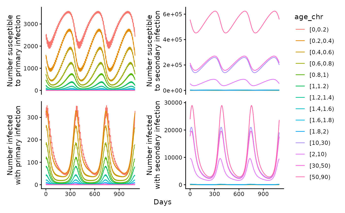
The incidence, detected incidence and prevalence are also calculated. To calculate the detected incidence age-specific detection probabilities are used, and in the default parameters we assume no one over the age of 2 years old is tested.

ggplot(data = out, 
       aes(x = time, y = DetIncidence)) +
  geom_line() +
  facet_wrap(~age_chr) + theme_classic() +
  ylab("Detected incidence") +
  xlab("Days")

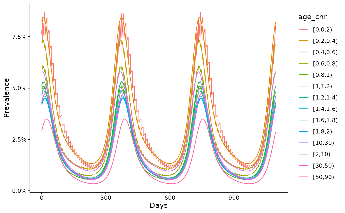
ggplot(data = out, 
       aes(x = time, y = prev)) +
  geom_line() +
  scale_y_continuous(labels = scales::percent) +
  facet_wrap(~age_chr) + theme_classic() +
  ylab("Prevalence") +
  xlab("Days")