In this vignette we will show how to calibrate the model to age-specific incidence data. To calibrate the model we vary the b0 (transmission rate coefficient), b1 (amplitude of seasonal forcing) and phi (phase shift of seasonality) parameters.
Simulating some synthetic data
We begin by simulating some data using the R/RSVsim_run_model.R function. To do so, we arbitrarily select a value of , value of and value of days. We then add noise to this count data by drawing random samples from a negative binomial distribution with greater variance than the poisson distribution and a mean equivalent to the simulated incidence values.
age.limits <- c(seq(0, 5, 1), seq(10, 70, 20))

contact_population_list <- RSVsim_contact_matrix(country = "United Kingdom", age.limits = age.limits)
#> Warning in pop_age(survey.pop, part.age.group.present, ...): Not all age groups represented in population data (5-year age band).
#>   Linearly estimating age group sizes from the 5-year bands.

parameters <- RSVsim_parameters(overrides = list("b0" = 0.15,
                                                 "b1" = 0.25,
                                                 "phi" = 10),
                                contact_population_list = contact_population_list)

model_simulation <- RSVsim_run_model_dust(parameters = parameters,
                                          times = seq(0, 365 * 4, 0.25),
                                          warm_up = 365 * 3,
                                          init_conds = NULL,
                                          cohort_step_size = 10
                                     )

set.seed(123)
data <- data.frame(time = model_simulation$time,
                 incidence = as.integer(rnbinom(n = nrow(model_simulation), mu = model_simulation$Incidence, size = 30)),
                 age_chr = model_simulation$age_chr) |>
  subset(time %% 10 == 0)
Likelihood calculation
The R/RSVsim_calibration_parameters.R function can be used to obtain the age groupings, times and parameter values required for each dataset of age-specific incidence data within a list of data frames. Each data frame must contain a time (numeric), incidence (integer) and age_chr (character) columns. age_chr is the age grouping. The overrides argument can be used to specify changes to the fixed parameter values. The parameters we want to fit must be named as a vector of characters in the fitted_parameter_names argument. In this case we fit b0 and b1 only.
We assume that the incidence, , in age group, , at time, , is Poisson distributed and calculate the log-likelihood in the R/RSVsim_log_likelihood.R function: , where is the corresponding model simulated incidence.
fixed_parameter_list <- RSVsim_calibration_parameters(data = data,
                                                      fitted_parameter_names = c("b0", "b1"),
                                                      overrides = list("phi" = 10),
                                                      country = "United Kingdom",
                                                      warm_up = 365 * 3,
                                                      cohort_step_size = 10)
#> Warning in RSVsim_contact_matrix(country = country, age.limits = age.limits):
#> polymod age groupings only go up to 75. Age limits above this have therefore
#> been omitted.
#> Warning in pop_age(survey.pop, part.age.group.present, ...): Not all age groups represented in population data (5-year age band).
#>   Linearly estimating age group sizes from the 5-year bands.

RSVsim_log_likelihood_dust(fitted_parameters = c("b0" = 0.15, "b1" = 0.25),
                           fitted_parameter_names = fixed_parameter_list$fitted_parameter_names,
                           fixed_parameters = fixed_parameter_list$fixed_parameters,
                           data = data,
                           times = fixed_parameter_list$times,
                           warm_up = fixed_parameter_list$warm_up,
                           cohort_step_size = fixed_parameter_list$cohort_step_size
                           ) |> print()
#> [1] -2858.713
Maximum likelihood estimation
In the R/RSVsim_max_likelihood.R we use the nmlinb function https://github.com/SurajGupta/r-source/blob/master/src/library/stats/R/nlminb.R to estimate the parameters that give the maximum likelihood. The lower_ll and upper_ll arguments specify the lower and upper parameter limits. scale_parameters is a boolean indicating whether the parameters should be scaled between 0 and 1.
fitted_values <- RSVsim_max_likelihood_dust(data = data,
                                            fitted_parameter_names = fixed_parameter_list$fitted_parameter_names,
                                            fixed_parameters = fixed_parameter_list$fixed_parameters,
                                            times = fixed_parameter_list$times,
                                            cohort_step_size = fixed_parameter_list$cohort_step_size,
                                            init_conds = NULL,
                                            warm_up = fixed_parameter_list$warm_up,
                                            scale_parameters = FALSE,
                                            lower_ll = c(0.01, 0),
                                            upper_ll = c(5, 1)
                                            )

print(fitted_values$par)
#> [1] 0.1486841 0.2483170
We can then use these fitted parameter values to simulate transmission.
parameters_fit <- RSVsim_parameters(overrides = list("b0" = fitted_values$par[1],
"b1" = fitted_values$par[2],
"phi" = 10),
contact_population_list = contact_population_list)
model_simulation_fit <- RSVsim_run_model_dust(parameters_fit,
times = seq(0, 365 * 4, 0.25),
warm_up = 365 * 3,
init_conds = NULL,
cohort_step_size = 10)
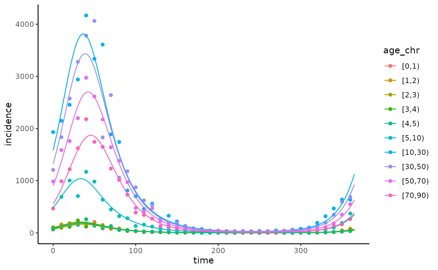
ggplot(data = data |> dplyr::mutate(age_chr = factor(data$age_chr,
levels = c("[0,1)", "[1,2)", "[2,3)", "[3,4)", "[4,5)", "[5,10)", "[10,30)", "[30,50)", "[50,70)", "[70,90)"))),
aes(x = time, y = incidence, col = age_chr)) +
geom_point() +
theme_classic() +
geom_line(data = model_simulation_fit, inherit.aes = FALSE,
aes(x = time, y = Incidence, group = age_chr, col = age_chr)
) ## Bayesian parameter estimation To fit the posterior estimates of the
and
parameters we use the monty package to run Hamiltonian MCMC.
## Bayesian parameter estimation To fit the posterior estimates of the
and
parameters we use the monty package to run Hamiltonian MCMC.
# prior_functions_list <- vector(mode = "list", length = 1)
#
# prior_functions_list[[1]] <- function(x){
#   return(dgamma(x, shape = 10, rate = 20, log = TRUE))
# }
#
# prior_functions_list[[2]] <- function(x){
#   return(dgamma(x, shape = 5, rate = 20, log = TRUE))
# }
#
# prior_functions_list[[1]] <- function(x){
#   return(dgamma(x, shape = 1, rate = 1/180, log = TRUE))
# }
#
# nchains <- 4
#
# initial_mat <- matrix(NA, nrow = nchains, ncol = 1)
#
# for(i in 1:nchains){
#   #initial_mat[i, 1] <- runif(1, min = 0, max = 10)
#   #initial_mat[i, 2] <- runif(1, min = 0, max = 1)
#   initial_mat[i, 1] <- runif(1, min = 0, max = 365.25)
# }
#
# fitted_parameter_names <- fixed_parameter_list$fitted_parameter_names
# fixed_parameters <- fixed_parameter_list$fixed_parameters
# times <- fixed_parameter_list$times
# cohort_step_size <- fixed_parameter_list$cohort_step_size
# init_conds <- NULL
# warm_up <- fixed_parameter_list$warm_up
#
# phi <- seq(-25, 375, 10)
#
# p_check <- rep(NA, length(phi))
#
# for(i in 1:length(phi)){
#   print(i)
#   p_check[i] <- RSVsim_posterior(fitted_parameters = phi[i],
#                              fitted_parameter_names = fitted_parameter_names,
#                              fixed_parameters = fixed_parameters,
#                              data = data,
#                              times = times,
#                              cohort_step_size = cohort_step_size,
#                              init_conds = init_conds,
#                              warm_up = warm_up,
#                              prior_functions_list = prior_functions_list,
#                              lower_ll = lower_ll,
#                              upper_ll = upper_ll)
# }